
The clock everyone starts by accident
Say you have an agent that looks up inventory, calls a tool to check a supplier's API, and then drafts a reply. You add prompt caching to the model call, because the same system prompt and tool definitions get sent on every turn. You measure the model call before and after: it used to take 900 milliseconds, now it takes 300. For this hypothetical case, that is a 66.7 percent reduction in the model-call interval.
Except nobody who uses the agent experiences that number. They experience the time between sending a request and getting a usable answer, and if the tool call now sits in a queue behind other tool calls, waiting two extra seconds for a busy downstream service, the user's wait went up while your model latency chart went down. Both numbers are true. Only one of them describes what the user felt.
This is the trap in the reader's task: locate the delay that matters before optimizing token generation. The mechanism problem isn't measurement error. It's an unstated decision about which interval counts as "the latency," made silently by wherever your stopwatch starts and stops.
Two quantities that are not interchangeable
User-visible time to first token runs from the user's request to the first rendered output token. Provider-side time to first token starts and ends at different boundaries; buffering, tool calls and rendering can separate the two. Time to accepted completion tells you how long until the task is actually done and the result is usable. These are different quantities in the same sense that a car's top speed and its time to destination are different quantities: a faster top speed doesn't guarantee you arrive sooner if you hit more traffic lights.
A related distinction from the caching lesson referenced in this course applies directly here: cached tokens still occupy context, so a cheaper request is not a larger memory (see the course's prompt caching lesson). The parallel claim for latency is that a faster model call is not a faster workflow. Speeding up a stage on the critical path can reduce total duration even if it is not the longest stage. You need to know the ordering and whether other stages changed.
Anthropic's engineering guidance on evaluating agents makes a related point about breaking a single aggregate into its parts: agent evaluation separates tasks, environments, trajectories and outcomes, and no single number can establish every operating requirement (Anthropic, "Demystifying evaluations for AI agents," https://www.anthropic.com/engineering/demystifying-evals-for-ai-agents, retrieved 2026-09-10). The same logic applies to timing. A single latency number, however precisely measured, cannot tell you whether the user's actual wait improved, because it collapses stages that behave independently.
Building the timeline
Here is the mechanism. Every agent turn has an arrival time, when the request lands. It may sit in a queue before anything starts. Then retrieval or context assembly happens. Then the model begins generating; its first generated token may be a tool call rather than output visible to the user. If the model calls a tool, that tool has its own duration, which might overlap with model generation or might block it entirely depending on your architecture. Finally, a result is accepted, either automatically or by a human reviewer.
The failure mode is treating "model call duration" as a proxy for any of the boundaries that actually matter to the user. Model call duration is a real, measurable interval. It is just not the interval a person waiting for an answer experiences.
Each arrow in that diagram is a segment you can, in principle, timestamp. The diagram shows the ordering assumed for this example; actual pipelines may overlap work or make several model calls.
Working the example all the way through
Take a hypothetical timeline, clearly invented for teaching and not a measured result from any system: arrival at 0ms, queue exit at 100ms, retrieval end at 400ms, model start at 400ms, first token at 600ms, tool end at 1500ms, accepted result at 1800ms.
From this hypothetical timeline, two numbers matter and they are not the same number. First-token latency is 600ms, the interval from arrival to the first visible output. User-visible completion is 1800ms, the interval from arrival to an accepted result. If your dashboard only reports the first number, you are reporting how long the user waits before something appears, not how long they wait before they can act on the answer.
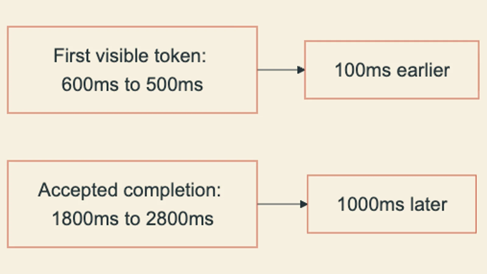
Now apply the caching change from the earlier scenario. Suppose a revised model configuration gets first token down to 500ms, a genuine 100ms improvement at that boundary, still a hypothetical figure. But the tool call, downstream of the faster model response, now ends at 2500ms instead of 1500ms, perhaps because the faster model is issuing tool calls that hit a rate-limited API more aggressively, or because saved time upstream simply shifted the queueing pressure downstream. Keep the 300ms finalization interval unchanged: acceptance now occurs at 2800ms. The complete task got slower even though first-token time improved.
This is not a contradiction. It's two different intervals responding to two different causes. The model change affected the model's own span. The revised run also has a slower tool stage; these invented timestamps do not establish why. A controlled experiment would be needed to attribute the change to caching. If your acceptance criterion is "the user got a useful answer," 1800ms beat 2800ms, and the caching change failed your actual promise even though it succeeded at the narrower thing you measured.
Timing your own process's calls, even accurately, tells you about that program's execution. It does not tell you what an external API, queue, or reviewer actually did on their side, and it is not evidence of production behavior at a supplier you don't control.
Here are the two complete hypothetical timelines. Tool end and accepted completion are separate timestamps.
| Boundary from arrival | Original | Revised |
|---|---|---|
| Arrival | 0ms | 0ms |
| Queue exit | 100ms | 100ms |
| Retrieval end and model start | 400ms | 400ms |
| First visible token | 600ms | 500ms |
| Tool end | 1500ms | 2500ms |
| Accepted completion | 1800ms | 2800ms |
Marking what you don't know
A realistic trace has gaps. Maybe you have solid timestamps for arrival and for accepted result, but no visibility into when the queue actually released the request, because that happens inside infrastructure you don't instrument directly. The honest move is to mark that interval as unknown on the diagram rather than to guess a value or, worse, to let two spans silently overlap as if they ran in sequence when they might have run concurrently.
This matters because overlapping spans, drawn as if sequential, will overstate total duration and hide genuine concurrency. If your tool call and a background retrieval step run in parallel, adding their durations invents a number nobody experienced. OpenTelemetry's generative AI semantic conventions, now maintained in their own repository, exist partly to standardize how spans and attributes get recorded so that this kind of ambiguity has a named place to live rather than getting lost in ad hoc logging (OpenTelemetry, "Generative AI semantic conventions," https://github.com/open-telemetry/semantic-conventions-genai, retrieved 2026-09-10). Exact attribute names and stability levels there are still moving, so check the current schema before you build a tracing pipeline against it, but the underlying discipline transfers regardless of the exact field names: label each span, record its start and end, and don't infer a boundary you didn't measure.
Running the experiment properly
A single hypothetical timeline demonstrates the mechanism but proves nothing about your actual system under load. To find out whether a latency change helps or hurts in practice, you need repeated trials, not one run.
Hold the request payload constant and run the same scripted request at one concurrent request, then at ten, with and without a shared limit on the tool queue. Using scripted, not live, model sampling for this control isolates queueing behavior from the model's own response-time variance.
For each run, log arrival time, queue exit, first-token time, and accepted-result time. Don't just log the final duration; you need the intermediate boundaries to tell which stage changed.
Look at the full spread of accepted-result times across trials before summarizing with any single number. A mean can look flat while the tail gets much worse. Include timeout and failure counts too; reporting only successful requests can hide the slowest failures. For end-to-end duration use timestamps on one clock where possible, or document clock synchronization and uncertainty across hosts.
If your commitment to users is about typical experience, look at the median. For a tail-latency target, check p95 or p99 completion time specifically, alongside first-token time, and report both with the trial count and percentile method you used.
If first-token time improves while p95 completion time worsens in a properly sized sample, the "faster model means faster workflow" inference fails, exactly as in the small hypothetical above, except now you have measured evidence for your own system instead of an illustrative timeline.
Check the decision
What would prove this argument wrong
This argument would fail if user-visible completion time and first-token time turned out to move together in practice, always, across architectures. They don't move together by structural necessity; tool calls, queues and review steps have their own durations, although upstream changes can affect their load, so there's no guarantee they track. But it's a fair challenge to ask for confirming measurement rather than taking the point on structure alone. The way to check is the load-matrix experiment above, run against your own agent, with real percentile reporting across enough trials to see the tail, not the three-point hypothetical used here for explanation. If, after running that experiment honestly, first-token time and completion time always move together for your particular pipeline, the two-clock distinction still holds conceptually, it just means your pipeline's stages happen to be tightly coupled, and that's a fact about your system worth stating explicitly rather than assuming for every agent.
A usable next step
Before touching model configuration to chase a latency number, draw your own timeline first: arrival, queue exit, retrieval end, first token, tool completion, accepted result. Mark every boundary you can actually timestamp and mark the rest as unknown. Decide, in writing, which interval is your promise to users. Then run the concurrency experiment above before and after any change, comparing full distributions rather than single before-and-after numbers. If you're already working through the caching material that raised this exact distinction between a cheaper call and a genuinely faster workflow, the next reading builds directly on it.
That lesson works through the companion distinction between cheaper token billing and larger context, using the same discipline of separating measurements rather than assuming one number stands in for another.