

Lucy has fine-tuned a model to work arithmetic problems. Its accuracy is around 80%. A second training stage, direct preference optimization, optimizes a reference-relative preference loss and nudges recorded accuracy upward. Can she report an improvement?
That question has two parts. First, what did the new objective reward? Second, how much evidence supports the accuracy difference? We implement both stages on a small base language model, follow the tokens that receive gradients, and inspect Rod's recorded T4 results. SFT produces a large measured improvement over the three-example base model. DPO's incremental gain remains unresolved.
Entry skills: Python, token probabilities and basic gradients. The shifted next-token targets are explained in the SFT section below. Output: a CPU experiment that changes the reply boundary and preference margin, followed by a short write-up separating the objective, heldout accuracy and uncertainty. You do not need a GPU for that route.
The guided notebook starts with saved measurements and a standard-library exercise. Its optional full route reproduces the original model training. The companion includes explicit PyTorch loops, original receipts and standalone figures.
Fix the task before choosing the objective
The prompt asks for one arithmetic operation per line, ending with Answer: <number>. For 45 + 87 * 9, the supplied solution is:
87 * 9 = 783
45 + 783 = 828
Answer: 828
The generator obeys multiplication precedence and uses three operands. It produces disjoint expression strings for 3,000 SFT problems, 1,000 preference-sampling problems, 300 development problems, 1,000 test problems and three demonstration examples. All splits come from fixed seeds; the receipt pins their hashes. Disjoint expression strings prevent this experiment's train/test duplication. They cannot establish that the pretrained model never encountered similar arithmetic.
The grader extracts the first integer after Answer: and compares it with the known answer. It does not validate every worked step or require an otherwise correct explanation. Even a reply with a wrong trace can receive credit for the final integer. Accuracy therefore measures this answer-extraction task, rather than verified reasoning.
We start from SmolLM2-360M, the base model, not its instruction-tuned variant. SFT uses full fine-tuning, one epoch, batch size 16 and learning rate . DPO starts from each resulting SFT checkpoint, uses two epochs, batch size 16, learning rate and . The earlier local MPS development-split calibration chose these settings; the T4 run reused them. Test comparisons did not choose a new learning rate.
The two base-model conditions differ in both examples and format: three worked examples in plain text versus zero-shot ChatML. Their 27.5% and 0.0% scores help locate the starting behavior. They do not isolate a single effect of the chat template.
SFT: predict the reply while reading the prompt
Let be a tokenized prompt and its supplied reply, including the closing turn token. The model reads the prompt and earlier reply tokens. Supervised fine-tuning minimizes their negative log-probabilities:
Here concatenates prompt and reply, contains reply target positions across the batch, and is their count. This implementation averages over scored tokens, rather than giving every differently sized example equal weight. Prompt tokens remain inputs; their labels are ignored as targets. They can still affect the reply predictions and the gradients flowing through the network.
The boundary is easy to misread after the causal shift. Use synthetic IDs to see it without downloading a model:
prompt = [10, 11, 12]  # includes assistant opening
reply = [20, 21, 2]    # ends with closing turn token
ids = prompt + reply
labels = [-100] * len(prompt) + reply
print(ids[:-1])     # [10, 11, 12, 20, 21]
print(labels[1:])   # [-100, -100, 20, 21, 2]
The last prompt input, 12, predicts the first reply token, 20. Masking that target would lose the first reply prediction. Scoring the first two targets would instead train on part of the prompt. Right-padding labels with -100 keeps padding out of the loss.
The actual loop makes the shift explicit:
loss = torch.nn.functional.cross_entropy(
    logits[:, :-1].float().reshape(-1, logits.size(-1)),
    labels[:, 1:].reshape(-1),
    ignore_index=-100,
)
SFT encourages the supplied continuation token by token. It neither compares that continuation with a rejected alternative nor directly optimizes the final-answer grader.
DPO: change a relative preference
For each of 1,000 fresh preference-sampling problems, each SFT model samples four replies at temperature 1. If a problem has both correct and incorrect replies under the answer grader, the code keeps one of each. Problems with only correct or only incorrect samples contribute no pair. Thus 1,000 problems does not imply 1,000 training pairs; the aggregate T4 receipt does not record the retained count.
Call the retained replies and , for chosen and rejected. Their sampled token IDs are preserved, including any generated closing token. Re-tokenizing decoded text could change the sequence being scored. The implementation sums reply-token log-probabilities:
This is a sum, not a per-token average; changing that operation changes the objective and its sensitivity to reply length. Prompt and padding targets are excluded with a shifted scoring mask, just as in SFT.
The reference is that seed's SFT checkpoint. Before DPO updates, the code scores every fixed chosen/rejected pair under the SFT model, saves those reference values and holds them constant. This avoids keeping a second model in memory. It works because these training pairs remain fixed.
Define the relative margin
The DPO paper (Rafailov et al., NeurIPS 2023) gives the reference-relative preference classification objective. For our fixed pair, the implemented loss is
At initialization, policy and reference are the same: and the loss is . Differentiating the scalar loss gives
The derivative is negative, so reducing the loss encourages a larger chosen-minus-rejected change relative to the reference. It does not require the chosen reply's absolute probability to rise. Neural parameters also couple many sequences; this scalar direction alone cannot predict heldout accuracy.
The loop uses stable log-sigmoid and summed reply log-probabilities:
margin = beta * ((pc - rc) - (pr - rr))
part = -torch.nn.functional.logsigmoid(margin).sum() / len(chunk)
part.backward()
pc and pr are policy scores; rc and rr are fixed reference scores. A 16-pair chunk is split into micro-batches of eight pairs. Each partial sum is divided by the whole chunk's pair count, gradients accumulate, and one clipped optimizer update follows. Averaging each micro-batch equally would misweight a shorter final micro-batch.
A better margin can accompany worse likelihoods
Take synthetic reference scores and . Suppose training lowers the chosen score by 1 nat and the rejected score by 3 nats. Then , so and the loss falls from 0.6931 to about 0.5981.
Yet the chosen reply's probability becomes times its reference probability. The rejected probability falls further, to . The preference improved relatively while both absolute likelihoods fell. These are synthetic scores illustrating the loss, not observed T4 model outputs.
Predict first: lower both reply scores. Which one must fall further for the preference loss to decrease?
Synthetic pair: fixed reference log-probabilities −10 (chosen) and −12 (rejected), with β = 0.1. These are whole-reply scores in nats, not token averages or recorded T4 results.
Margin 0.00 nats; βm = 0.00; loss 0.6931. Chosen probability is 1.000 times reference; rejected probability is 1.000 times reference.
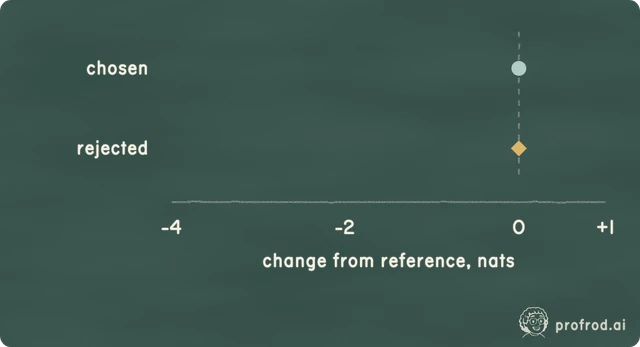
Solid sea-glass circle: chosen reply. Dashed brass diamond: rejected reply. Zero means no change from that reply’s reference score.
| Reply | Log-probability | Probability |
|---|---|---|
| Chosen | -10.00 | 4.540e-5 |
| Rejected | -12.00 | 6.144e-6 |
Other replies can receive the probability mass. These two replies do not exhaust the possible continuations. A lower pair loss does not establish better answer accuracy.
Worked counterexample, also available without JavaScript
Changes −1 and −3 give margin 2, loss 0.5981 instead of 0.6931, chosen probability ratio 0.368 and rejected ratio 0.050. Both probabilities fall; the rejected reply falls further.
Change the two policy scores while keeping the reference and fixed. The two replies are not an exhaustive distribution: probability mass can move to other replies. The relative margin and pair loss cannot tell you whether held-out answer accuracy improved.
A falling DPO loss establishes progress on the retained pair objective. A larger fraction of positive margins establishes ordering relative to the reference on those pairs. Neither quantity substitutes for correctness on heldout problems.
Predict the DPO gain
Ask what you would need to know about the items on which the two models disagree.
Check the prediction
Three positive point estimates do not settle it
Whether a gain that small is distinguishable from noise depends on the paired interval over the test items, and that depends on how many items the two models answer differently, not on the size or sign of the average gain. A small gain from a few items that always flip the same way can have an interval that excludes zero; the same gain from many items that flip both ways can have one that includes zero. Neither "clearly improves" nor "no effect" follows from the three gains. The next section gives the recorded interval.
What the T4 run measured
Rod's October 3 receipt records three training seeds on the same 1,000 test problems. Evaluation uses greedy decoding, a 64-token maximum and the answer grader described above.
| Condition | Seed 0 | Seed 1 | Seed 2 | Mean accuracy |
|---|---|---|---|---|
| Base, three examples | 27.5% | — | — | 27.5% |
| Base, zero-shot ChatML | 0.0% | — | — | 0.0% |
| Reply-only SFT | 79.2% | 81.9% | 80.2% | 80.43% |
| DPO after SFT | 79.9% | 82.0% | 80.8% | 80.90% |
Scroll horizontally to view columns.
SFT exceeds the three-example base model by 52.93 percentage points, with a recorded paired 95% interval of 49.87 to 56.00. It also passes the experiment's additional per-seed interval rule. This supports improved answer accuracy under the defined task and protocol; it does not prove that every worked step became correct.
DPO's seed gains over SFT are +0.7, +0.1 and +0.6 percentage points. Their mean is +0.47, with a recorded paired 95% interval of −0.63 to +1.57. The interval includes zero, and the receipt reports real: false. The incremental gain is unresolved. All three positive point estimates do not establish improvement, and the interval does not establish equivalence or zero effect.
Each line pairs one training seed. The seed-to-seed spread is larger than the incremental changes within seeds.
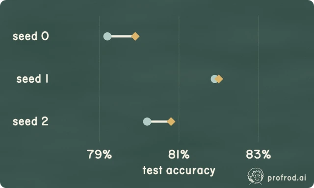
Sea-glass circles: SFT. Brass diamonds: DPO. These are point estimates on the same 1,000 items, without error bars.
| Seed | SFT | DPO |
|---|---|---|
| 0 | 79.2% | 79.9% |
| 1 | 81.9% | 82.0% |
| 2 | 80.2% | 80.8% |
Figure 1. Each line connects an SFT checkpoint with its DPO continuation. Sea-glass circles are SFT; brass diamonds are DPO. These are point estimates on the same 1,000 items, not confidence intervals. The seed-to-seed level changes are visibly larger than the incremental change within each seed.
Which uncertainty does that interval describe?
Let and indicate whether SFT and DPO, respectively, answer item correctly after training seed . The paired difference for an item is
The statistics code resamples the item index 10,000 times, retaining each item's paired, seed-averaged difference. It takes percentile endpoints from the resampled means. Pairing matters because both models see the same item; the difference depends on which items they disagree about, not just their separate total accuracies.
This interval addresses item-sampling uncertainty conditional on the three fixed trained seeds. The bootstrap does not draw new training seeds. The 3,000 seed-item evaluations are not 3,000 independent test problems. The per-seed table reports a separate source of variation; neither the pooled item interval nor three observed seeds precisely characterizes performance after a fresh training run.
The experiment's real flag requires the pooled interval to exclude zero and every individual seed's paired interval to exclude zero in the same direction. This is a stated agreement rule, not a calibrated guarantee about all future seeds. The full T4 receipt preserves its verdicts, but omits individual seed interval endpoints and raw correctness rows. We can verify the means and split hashes; we cannot recompute the T4 paired bootstrap from these aggregate scores.
Change the implementation contract and measure again
The original experiment includes three controls against the same-seed SFT model. They ask different questions: one changes training labels, and two change the evaluation prompt.
| Change relative to SFT | Mean accuracy | Difference, percentage points | Recorded 95% item interval |
|---|---|---|---|
| Include prompt targets in SFT loss | 77.77% | −2.67 | −4.07 to −1.33 |
| Add an unseen system prompt at evaluation | 80.33% | −0.10 | −0.70 to +0.50 |
| Remove assistant-opening tokens at evaluation | 80.77% | +0.33 | −0.10 to +0.77 |
Scroll horizontally to view columns.
The prompt-loss control trains the same kind of model but scores prompt targets too. That changes both the loss's terms and its token-count denominator. It allocates optimization effort to predicting the prompt's tokens as well as the supplied reply. The negative pooled interval supports lower answer accuracy for this fixed-seed comparison. It does not by itself isolate which mechanism caused the reduction.
The receipt still says real: false for prompt loss: the stricter per-seed agreement rule failed. This is compatible with a pooled interval entirely below zero. The supplied T4 receipt does not identify the failing seed interval; assigning it to a particular seed would invent evidence.
The two template-control intervals include zero. Their bounds describe the observed uncertainty under these prompts, this model and this task. We did not specify an equivalence margin, so neither establishes that the mismatch has no effect. A narrow arithmetic prompt also cannot establish robustness to arbitrary changes in the chat format.
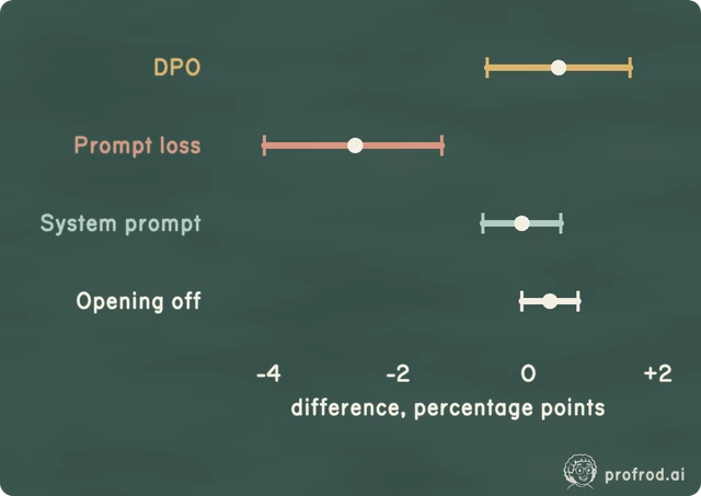
Recorded 95% paired item-bootstrap intervals, each relative to SFT. The three training seeds stay fixed.
| Change | Mean | 95% interval |
|---|---|---|
| DPO | +0.47 | −0.63 to +1.57 |
| Prompt loss | −2.67 | −4.07 to −1.33 |
| System prompt | −0.10 | −0.70 to +0.50 |
| Opening off | +0.33 | −0.10 to +0.77 |
The DPO interval includes zero. The pooled prompt-loss interval is negative, while its additional per-seed agreement rule fails. Neither result establishes equivalence.
Figure 2. Dots are mean accuracy differences; horizontal lines are recorded paired 95% bootstrap intervals over test items. The dashed vertical line is zero. All intervals condition on the same three training seeds. Prompt loss's pooled interval is negative even though the additional per-seed agreement rule fails. The other three intervals include zero.
Run the short experiment and write the claim
Use the notebook's first cells, or run the companion locally with Python's standard library:
python sftdpo_mechanism_v1.pyThe helper checks the original T4 receipt's SHA-256, regenerates all five split hashes from the task code, verifies the recorded means and prints the synthetic mask/margin examples beside the saved comparison. It downloads no model, calls no API and performs no training.
Identify the input position that predicts the first reply token. Turn on prompt_loss=True and explain which extra targets receive loss.
Start with drifts (0, 0), then try (-1, -3) and (-3, -1). Explain both losses and both absolute probability changes.
State the DPO gain and interval in percentage points. Identify what the item bootstrap resamples and what remains fixed.
Describe the objective, implementation check, measured outcome and limit. Explain why real: false means different things for DPO and prompt loss here.
Check the mechanism and bound the conclusion
The shifted reply-only labels are [-100, -100, 20, 21, 2]; input 12 predicts reply token 20. Including prompt targets replaces the first two ignored labels with 11 and 12. Drifts (-1, -3) give scaled margin +0.2 and loss about 0.5981; reversing them gives −0.2 and about 0.7981. Both replies lose absolute probability in either intervention.
A defensible conclusion is: “On the fixed 1,000-item arithmetic test, mean T4 accuracy rose from 80.43% after SFT to 80.90% after DPO. The +0.47 percentage-point difference has a recorded paired item-bootstrap interval of −0.63 to +1.57, conditional on three training seeds; an incremental gain is not established. The objective favors relative pair preference, which can improve while chosen likelihood falls. Raw T4 item correctness and per-seed interval endpoints were not supplied, so these intervals are reported rather than independently recomputed.”
Optional full reproduction and provenance
The original T4 run used float32 weights, activations and AdamW state. Recorded SFT peaks were 7.62–7.63 GiB; the largest recorded DPO peak was 9.71 GiB. SFT training took about 3.23 minutes per seed and DPO's recorded training sections about 3.83–4.00 minutes per seed. The 23 recorded sections total 41.42 minutes, excluding setup and other notebook overhead. This measured session supports feasibility on that T4; it does not guarantee free GPU availability or the same timing elsewhere.
The earlier MPS pilot and development calibration remain separate evidence. They are useful for inspecting raw generations and implementation diagnostics, but their item-level outputs cannot fill gaps in the T4 receipt. No new GPU training is needed to understand or report the comparison above.
Receipt provenance and reproducibility
The original operator download is preserved unchanged as receipts/colab/sftdpo-full-20261003.json, 9,378 bytes, SHA-256 a32dfc7af44c70d627d83009fd5db2e9f90839a10ec5b5893130aa8b94b23ca7. It records October 3, 2026, Tesla T4, Python 3.13.15, PyTorch 2.11.0+cu130, transformers 5.18.0, tokenizers 0.23.2, CUDA 13.0 and driver 580.82.07. SmolLM2-360M is pinned to revision f8027fd0eaeea54caa13c31d31b9fdc459c38b49, with Apache-2.0 model licensing reported in the receipt.
Data is generated locally by the repository's MIT-licensed task code, with seed 20261002 and no dataset download. Receipt hashes pin all five splits. The receipt reports USD $0 on local/free Colab compute and no API calls. The aggregate receipt retains per-seed accuracies, pooled intervals, verdicts, timings and allocated-memory peaks. It does not retain T4 correctness strings, sampled pairs, generation texts, training curves or per-seed interval endpoints. Neither the figures nor the CPU helper reconstruct those missing observations. The figures draw recorded aggregate values; the helper's IDs and log-probabilities are explicitly synthetic.
The optional GPU route uses the original sftdpo_run_v1.py, sftdpo_task_v1.py and sftdpo_stats_v1.py with pinned model/data settings. Notebook v2 places the short CPU route first and retains the original full experiment afterward. Original notebook v1 and earlier MPS receipts stay available as historical artifacts.
Lucy can now report a strong SFT result and an unresolved incremental DPO result without confusing either with the preference loss. For the next measurement habit, work through evaluation variation across repeated runs: the unit you resample must match the claim you want to make.
Compare repeated evaluations and distinguish variation across cases from variation across runs.